Math behind (convolutional) neural networks
In this article we will derive the basic math behind nerural networks. Later we will adapt the equations for convolutional neural networks. I’ve done this by hand for my super-resolution using neural networks project, so that you don’t have to.
If you are looking for practical tips about implementing neural networks, you should check out my other article - “Writing neural networks from scratch - implementation tips”.
Chain rule
Do not skip this part. Whole article is just application of this rule and following graphic representation helps a lot.
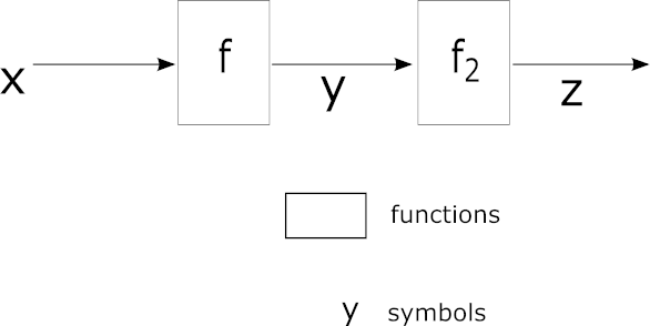
Example combination of functions f, f2 that we want to calculate partial derivatives from
We have . Let say we also have some (requirement: z is function of y) and we know the function f. We can calculate using following formula:
Now look again at the picture above and locale each variable. What is ? It’s just . Since we know f we should be able to provide . Now, having removed all math obstacles, let see how we can apply this to neural networks. First we are going to supply some nomenclature.
Dictionary
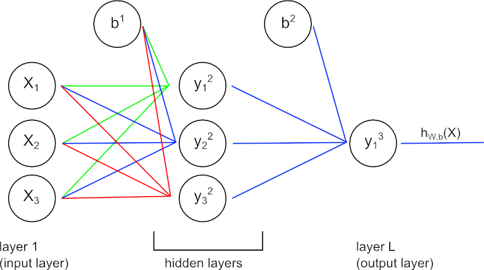
Example of neural network
- l - layer index, especially l=1 for input layer and L for last layer
- - hypothesis produced by the network. We are going to assume that
- node/unit - single neuron (symbols: X for nodes in input layer, otherwise)
- - number of nodes on layer l
- - activation function
- - value of node on layer l before application of activation function (see image below)
- - value of node on layer l after application of activation function: (see image below)
- - weights between i-th node on layer l and j-th node on layer l+1. Take a notice of order of ji - it’s reversed to what You would expected. It is popular notation in all neural networks descriptions.
- - biases used during forward propagation
- - learning rate (hyperparameter)
- - error term of j-th node of l-th layer
- cost function J - how good the network’s output maps to ground truth
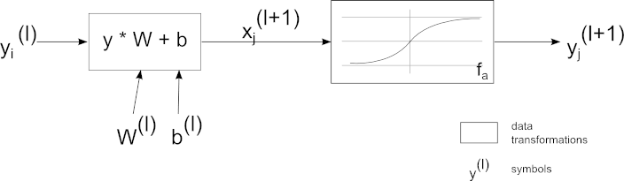
Relation between 2 nodes on successive layers.
Forward propagation in fully connected neural networks
We are going to use the following formulas:
How bad is it?
During reinforced learning it’s critical to be able to judge the results of algorithm. Let’s say that we have a sample (Y,X), where Y is ground truth and X is input for our neural network. If we do forward propagation sequentially across all layers with some weights and biases we will receive hypothesis: . We define cost function as (one-half) squared error:
In layman’s terms we measure difference between what we expected and what the algorithm has given, we square it and take half. Taking half of the result will come handy when we will calculate the derivative. It is also popular to add weight decay term to this formula, but we will keep things simple.
Training algorithm
Our goal is to minimize and to do that we will use gradient descent(GD) algorithm. Requirements of GD: function F is both defined and differentiable at least in neighbourhood of some point p. If we have a gradient at p we know in which ‘direction’ we can move so that the function increases it’s value. If we move in negative direction the opposite should be true: . For this to work we write GD as:
As You can see we subtract to move in direction that should give smaller . The (greek letter eta) determines how fast we are getting closer to the local minimum. If is too big, we will constantly miss it, if it is too small we will have to repeat the process a lot. You may remember from the symbols table that represents hyperparameter called learning rate.
We will update parameters with every epoch according to the following formulas:
It’s nothing more then applied gradient descent algorithm. The thing is that we have to update value for every parameter, for every layer in our network. We already have and (these are the current values), is either a constant or we have some separate algorithm to calculate it. How to find and ? The solution is to use the backpropagation algorithm.
Backpropagation algorithm
Last layer deltas
For each node we can calculate how much “responsible” this node was for the error of our hypothesis. These are so called deltas / error terms. We will use to describe error term of j-th node of l-th layer. Let’s think about deltas for last layer. If we are using squared error as the cost function we have:
Do You see how expresses responsibility of j-th node for the error? The term comes from the that we have to include - it is one of the rules of calculating derivatives. We can use this formula to calculate deltas for all nodes in last layer.
It is important to see that we are calculating derivative w.r.t. , not .
Calculating remaining deltas
Sadly, calculations of deltas for other layers is a little bit more complicated. Let’s look again on the image of forward propagation between 2 nodes on successive layers:
Relation between 2 nodes on successive layers. Please refer to dictionary for explanation of the symbols.
Let’s assume that l is the layer before the last (). We have just provided equations for . After investigating the image above it turns out that we can use chain rule to provide formula for . We are going to do this in several steps. First observation:
This is not entirely correct. During forward step our node contributes in some degree to values of all nodes in layer l+1. As a consequence, in backpropagation we have to sum over all nodes in l+1. If is number of nodes in l+1 then:
On previous image we focused only on 2 nodes as it makes easier to derive formulas. In reality, every node contributes to values of all nodes on next layer.
Remember when I said that in deltas we were calculating derivative w.r.t. , not ? This applies here too. We have to use chain rule once more:
If then . We can use this the equation to calculate deltas for all nodes on other layers.
Derivative of J w.r.t to parameters
We have calculated deltas, now how does this help with parameters? Take a look once more on this image:
Relation between 2 nodes on successive layers. Please refer to dictionary for explanation of the symbols.
This should be simple:
and
All this because . I will leave calculating derivative of w.r.t each and to the reader.
With deltas we had and now we have . As You can see we use deltas in both of these expressions - that’s why we have calculated them!
Backpropagation in batch
Instead of updating parameters after each example it is more common to take average from the batch of m samples like this:
and
TL;DR
- Calculate deltas for each output unit (ones in last layer):
- For each unit in other layers calculate deltas (do it layer by layer):
- Calculate the derivatives for all weights and biases:
Now it’s time for part II.
Backpropagation in Convolutional Neural Networks
Main difference between fully connected and convolutional neural networks is that weights and biases are now reused.
TL;DR: You have a kernel (that actually consists of weights!) and You convolve it with pixels in top-left corner of image, then with pixels a little bit to the right (and so on), later repeat this in next row (and so on). Since we apply same kernel several times across the image, we effectively share kernel (therefore - weights).
Weights sharing in CNN. For each node on next layer the kernel stays the same, but input units change
Another thing we are not going to talk about is pooling.
Dictionary - CNN
- and - size of first 2 dimensions of the layer.
- - feature maps/filters for layer n. Creates layer’s third dimension - this means each layer has units.
- - spatial size of the kernel.
- - this is how we are going to index weights now. Each kernel has dimensions . There are kernels between each layers.
is activation function, is spatial size of kernel.
Size of the layers
If You have worked with image kernels before You know that it is a problem to handle pixels that are near the edges. Common solutions are to pad the image with zeroes around the borders or make each consecutive layer smaller. In latter case, we can determine size of layer’s first 2 dimensions with following formulas:
In case of 3 layers the output has following sizes when compared to the input:
Layer’s third dimension is the number of feature maps () for this layer.
Forward propagation
Based on reasons stated above:
Value ranges:
There are other ways to write this equations, but this one is IMO the simplest.
Deltas
Formula for deltas on last layer stays the same. As for everything else..
During forward pass we had summations like: . As You may have guessed, during backpropagation we will have something similar:
Previously, when calculating we used:
- derivative of this node’s value: ,
- all weights connected to x^{(l)}_i$$: $$W^{(l)}_{ji},
- for node at the other end of this weight
Turns out the only changes are the sums and indexes. Before, we summed over all nodes in next layer (it was ‘fully-connected layer’ after all), now we only interact with handful of nodes. Let’s write what is what:
- - derivative of activation function at current node
- - propagation weight between and
- - error term for . Also, since You have to do bounds check. For example, take nodes in bottom right corner of layer l: . This particular node will be used during forward pass only once (per feature map in ).
Sometimes it is written as . I’m not sure, but this may be a matter of indices. The minus since we have and we asking: ‘which affected us with w[a,b,-,-]?‘.
Value ranges:
Parameters
The key now is to follow the sentence from TL;DR in CNN - forward propagation:
‘Since we apply same kernel several times across image, we effectively share kernel (therefore - weights).’
More specifically, we are sharing each weight times. Now, during backpropagation we add all this contributions:
and
Summary
Hopefully notes presented here helped You understand neural networks better. If You know how the equations were created You can adapt them to any use case.
If you are looking for practical tips about implementing neural networks, you should check out my other article - “Writing neural networks from scratch - implementation tips”.