Writing neural networks from scratch - implementation tips
Judging by the number of new articles, neural networks were popular in recent months. And not only because Google, Netflix, Adobe, Baidu, Facebook and countless others has been using them. There are many hobbyists playing with machine learning too. After seeing amazing examples of what is possible I decided to create my own neural network. This article presents my findings. I hope You will find it useful.
If you are also interested in derivation of neural network equations, I’ve also got you covered. Check out “Math behind (convolutional) neural networks”.
Why not use Caffe / Torch7 / … ?
Using neural network frameworks have numerous advantages: they can provide minimum viable product faster, offer shorter training time, are thoroughly tested, have good documentation and You can always ask for help/submit issue in case of problem. Why would one want to do it all by hand? Let’s see:
- complete understanding of underlying mechanism – even with solid theoretical understanding there are always problems that manifest only in practice
- math – from raw equations to working prototype - how cool is that?
- more control over hardware
- interesting use case for GPU
- it’s fun!
My project
Throughout this post, I will be referring to my latest project: super-resolution using neural networks. The original paper Image Super-Resolution Using Deep Convolutional Networks - SRCNN was written by Chao Dong, Chen Change Loy, Kaiming He, Xiaoou Tang.
Super-resolution in itself is quite simple problem: how to make image bigger without losing much quality. It’s a popular question in computer vision, so there are quite a few methods to achieve such effect. I should point out that while there are infinitely many solutions, we -as humans- can instinctively determine if result is better. There are also special metrics (e.g. PSNR and SSIM) used for more systematic approach.

From left to right: ground truth, scaling with bicubic interpolation, CNN results.
My implementation was a simplified version of SRCNN. While number of layers and kernel sizes are still the same, due to performance constraints I’ve reduced number of feature maps for layers 1 & 2 by half. I also didn’t have enough time to wait for epochs for network to converge.
General tips
Common problems
Biggest problems that I’ve encountered:
- math
- hyperparameters tuning
- limited resources resulting in app crash
- training takes a lot of time
- getting optimal training samples
- parallel, asynchronous code execution on GPU
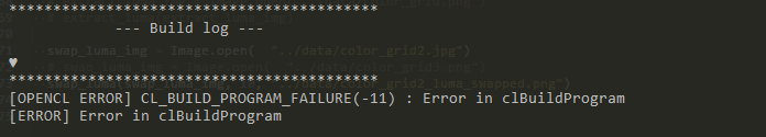
- GPU driver errors
Throughout the article I will give You some tips how to best approach all of them.
Supporting batching
During training You will operate on multiple samples, and -arguably- during normal usage this will also be the case. It is worth thinking how this aspect should be reflected in the design of the application. This is probably one of the most important architectural decisions You will make.
Advantages of processing images one by one:
- much easier to write
- can lazily allocate memory
- each kernel contains just straightforward implementation of math equations
- easy to test
When it comes to batching (each kernel operates on multiple images in a huge multigigabyte array):
- much more optimal GPU usage - e.g. more blocks per multiprocessor mean that we can easier hide memory access latency
- better performance - in my case it’s 2x faster, but that’s a low-end
- requires careful memory allocations (e.g. we have to place all images in one big array and then calculate offsets if want to get to particular image)
- calculating offsets in kernel while quite simple has to be correct
- hard to debug
- makes it easy to split epoch into mini-batches, which lowers the memory usage (more on that later)
Converting the neural network to support batching is quite complicated. If You find yourself in similar position I recommend first tuning the API to work on an array (with a single image for now), then test. Then switch the memory layout on GPU to a single block and test. After that execute kernels with all images at once. Turns out the last step can be done quite easily: You just need to add additional work dimension and in global_work_size, set it to number of images and to 1 in local_work_size. Other way is to add loop inside the kernels. This is probably even faster, since for multiple images You only load weights once.
uint sample_id = get_global_id(2);...#define IMAGE_OFFSET_IN (sample_id * PREVIOUS_FILTER_COUNT * input_w * input_h)#define IMAGE_OFFSET_OUT (sample_id * CURRENT_FILTER_COUNT * out_size.x * out_size.y)
Fragment of my forward kernel.
What to log?
Everything that is needed to reproduce results. This includes hyperparameters, parameters, pre and postprocessing methods, seeds, training/validation set split etc. Good idea is to use Git for settings/result storage but I’ve found that file based management suits me better. It is not necessary to log everything. For example why would You need detailed statistics about each epoch? Another case is when calculation of certain value show up during profiling. As long as You can reproduce the execution and have the crash log it’s often enough. On the other hand displaying learning progress once in a while is handy.
Since the data is heavily restricted to set of training samples and we are crunching numbers with amazing speed the failures do not happen often. On unrelated note Nvidia’s driver sometimes allows out of bounds access which manifests itself when You least expect it.
Choosing training samples
If there is standard sample set for Your domain use it. Good example is MNIST for handwritten numbers. Generating samples by hand is actually quite complicated. When I started I took small patches from random images and hoped my program would infer some general rules that would make it extremely universal and flexible. This was not a case. Fortunately, at least I was able to see that the network works (feature maps for first layer had familiar shapes of gaussian/edge kernels). I’d switched to images based on comics/vector graphic and received something recognisable much faster. Also important is the number of used samples and training/validation set split. With e.g. 200 samples at Your disposal and 80/20 split only 40 images will be used to measure model’s progress. This will attribute to huge variance. To compare: MNIST consists of over 60,000 images while ImageNet over 14,000,000.
“The size of training sub-images is fsub = 33. Thus the 91-image dataset can be decomposed into 24,800 sub-images, which are extracted from original images with a stride of 14.”
- Chao Dong, Chen Change Loy, Kaiming He, Xiaoou Tang: “Image Super-Resolution Using Deep Convolutional Networks”
There is also an excellent article written by Andrej Karpathy: „What I learned from competing against a ConvNet on ImageNet” that highlights some problems related to gathering samples. One solution is to use services like Amazon Mechanical Turk that allows to commision tasks that require human input.
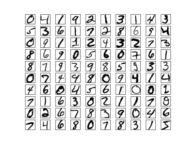
MNIST samples. Image taken from Michael Nielsen’s “Neural Networks and Deep Learning”. Distributed under MIT Licence.
Tests
Tests are necessary to check if math is implemented correctly, but is not only reason why You should write them. Beside usual suspects (ease of refactoring, better code design with isolated features, documentation through usage example etc.) it is important to test the application under heightened load. For example each OpenCL kernel on Windows has to finish in about 2s. If it takes longer then that the OS will decide that GPU is unresponsive (“Display driver stopped responding and has recovered”). I’ve used 2 separate test cases – one for correctness, one just uses a lot of data and checks if app crashes.
Linux also has similar limitation and on both systems it can be removed. Another solution is to use 2 graphics cards – one as system GPU, other for calculations.
It is also profitable to think how we would design testing framework. Of course we could use standard frameworks, but creating our own is quite simple and may suit our requirements better. Our kernels are quite simple data transformations so making the test data-driven is a good choice. Take a look at this file that defines all test cases for forward execution phase. By adding another entry I can easily create more tests, without even touching C++. Use scripts to generate test data e.g.:
def convolution(x, y, spatial_size, values):for dx in range(spatial_size):for dy in range(spatial_size):yield dy,dx,values[x+dx][y+dy]def forward(input,weights,bias,spatial_size,width,height):output = []for y in range(height):for x in range(width):tmp = 0for (dx,dy,input_value) in convolution(x,y,spatial_size,input):tmp += input_value * weights[dx,dy]output[y][x] += activation_func(tmp + bias)return output
2D convolution. Feature maps left as an exercise for reader
Since it is an offline tool the performance does not matter. Both R and MATLAB have convolution build-in, but it may require a little bit of juggling to convert Your data to suitable format.
Documentation
When looking through many open source projects I have a feeling that this step is just a personal preference. Many editors offer tools that can ease the task and it only takes a couple minutes, so why not? Anyway, I highly recommend to write down which kernel uses which buffers. It’s probably the best description of system one could have.
| Kernel | Buffers |
|---|---|
| forward propagation | in: weights, biases, previous layer output out: layer output |
| mean square error BLOCKING | in: ground truth luma, CNN output luma out: float |
| in: ground truth luma, CNN output luma out: | |
| in: , layer output, weights out: | |
| backpropagation | in: , layer output out: , |
| update parameters | in: , out: weights, biases inout: , |
| extract luma | in: 3 channel image out: single channel image |
| swap luma | in: 3 channel image, new luma out: new 3 channel image |
| sum BLOCKING | in: buffer with numbers out: float |
| subtract from all | inout: buffer with numbers |
My app
Useful scripts
C++ is quite low level language. It would be counterproductive to use it for everything, so I’ve switched to Python for some high-level operations like:
- managing backups
- scheduling
- high level debugging e.g. drawing feature maps
- generating reports
- creating test data
- creating training samples
List of scripts that I’ve used (feel free to reuse them):
- generate_training_samples.py - generate ready to use training samples based on images from provided directory
- weights_visualize.py - present weights as images
- profile.py - measure execution time or time spent per OpenCL kernel
- schedule_training.py – user can specify number of epochs or duration in minutes
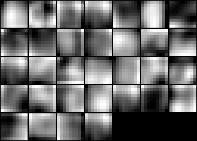
Drawing of weights for first layer. There are some gradients visible, but nothing interesting in particular (at least for now).
It’s also worth mentioning that You can hardcode some values into scripts and then change them without recompiling. It makes managing the configuration through separate folders easy as You can just copy the scripts and switch the values.
Did You know that copying file in python is one-liner (
shutil.copy2(src_file_path, dest_file_path))? Use it as simple backup system.
I highly recommend to write separate scheduling script. Some basic functionality should include e.g. ability to specify for how long to train (both by number of epochs and by duration), stop/resume, logs and backup management. Logging itself can be implemented as redirecting from sysout to file (although this solution has a lot of disadvantages).
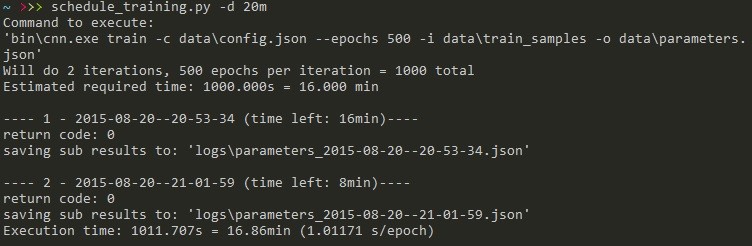
Scheduling script example
Separate parameters from hyperparameters
While not critical, in my opinion this step is quite important. Every change to hyperparameters directly affects parameters that You will receive, so –including backup- You will probably have quite a lot of files. Efficiently managing data is a skill on it’s own. This will come hand if You decide to create separate schedule script.
Optimization tips
In this part we will see how to make neural networks faster. The easiest way to improve performance is to study existing implementations, but -personally- I’ve found them quite hard to read. This chapter will be just about my personal observations since I’m not GPU architecture expert.
Also, AWS offers GPU instances (both On-Demand and Spot) that are quite popular. AWS offers subpar performance compared to e.g. TITAN X / GTX 980, but should be still quite fast. It’s perfect entry level option that does not require massive investment upfront.
Profile
One of the most important thing about profiling code is IMO to make it simple. Having to configure and run external program is often too much hassle. Sure, to closely investigate a bottleneck some additional information may be required, but a lot can be shown just from comparing 2 timer values. Writing separate profiling script makes it also easy to generate reports.
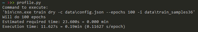
Quick and easy profiling. Run this program after each change to verify regressions.
Profiling OpenCL – simple way
The simplest way is to measure time spent per kernel. Fortunately OpenCL provides us with clGetEventProfilingInfo that allows us to inspect time counters. Call clGetDeviceInfo with CL_DEVICE_PROFILING_TIMER_RESOLUTION to get timer resolution.
For
clGetEventProfilingInfoto work You have to setCL_QUEUE_PROFILING_ENABLEflag duringclCreateCommandQueue.
Code sample (it slows down execution a lot):
cl_event kernel_ev;clEnqueueNDRangeKernel(..., &kernel_ev); // call kernelif (is_profiling()) {clWaitForEvents(1, &kernel_ev);cl_ulong start = 0, end = 0;clGetEventProfilingInfo(kernel_ev, CL_PROFILING_COMMAND_START, sizeof(cl_ulong), &start, NULL);clGetEventProfilingInfo(kernel_ev, CL_PROFILING_COMMAND_END, sizeof(cl_ulong), &end, NULL);execution_time[kernel_id] += end - start;}
After each kernel wait for it to finish and then retrieve the timestamps
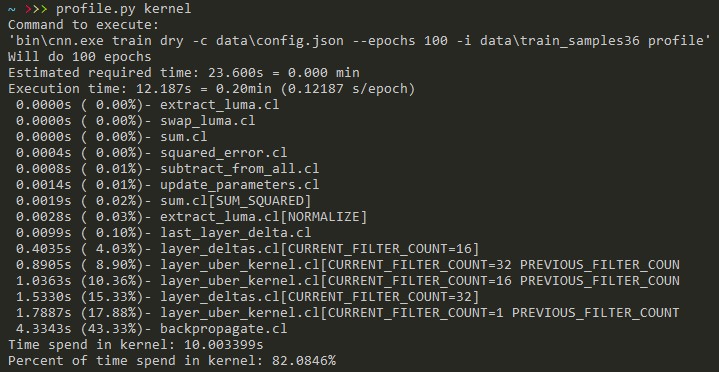
Time spent per kernel. Compile-time macros are also provided
Profiling OpenCL – Nvidia Visual Profiler
James Price has written an excellent article on getting nvvp to display OpenCL profile data. All that is needed is to set COMPUTE_PROFILE environment variable. You can also provide config file.
> set COMPUTE_PROFILE=1> set COMPUTE_PROFILE_CONFIG=nvvp.cfg> cat nvvp.cfgprofilelogformat CSVstreamidgpustarttimestampgpuendtimestampgridsizethreadblocksizedynsmemperblockstasmemperblockregperthreadmemtransfersize> bin\cnn.exe train dry -c data\config.json --epochs 100 -i data\train_samples36
You can create script from this
NVVP logs every single kernel invocation, so try to provide representative, yet short name for every kernel function.
Available information includes e.g.:
- occupancy
- number of registers used per work item
- shared memory per work group
- memory transfers size & bandwidth between host and GPU
- detailed timeline that marks start and end of each event
Use CodeXL for AMD devices.
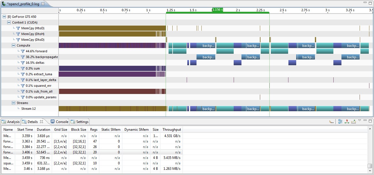
Nvidia Visual Profiler timeline view. On the left side we can see images being loaded to VRAM. Single epoch has been marked - it took 1.156s.
Remove blocking operations
The biggest change in performance in my case was due to removal of blocking operations like:
- clFinish
- clWaitForEvents
- clEnqueueReadBuffer
- clEnqueueReadBufferRect
- clEnqueueReadImage
- clEnqueueWriteBuffer
- clEnqueueWriteBufferRect
- clEnqueueWriteImage
- clEnqueueMapBuffer
- clEnqueueMapImage
Read, write and map operations should be used in non-blocking mode. Still, data transfer from host to GPU may be quite expensive. I was lucky to have all my data fit into the memory at once. If this is not possible, try to minimize the amount of data that is exchanged. You can pack it more effectively (e.g. half floats), but this is fairly low-level change. Another idea is to use memory pools. For example: the first half of images goes through every pipeline step, writes gradients and -only after it is done- the second half is executed. This can effectively cut the memory requirements in half since majority of VRAM is allocated to hold sub-step results (layer’s outputs, deltas). Also changing the number of this ‘mini-batches’ provides additional control over the execution. If the GPU usage is too high increasing this factor can effectively throttle the program.
Hardcode constants
And by hardcode I mean provide them at compile time as macros. This allows for:
- arrays in kernels
- better compiler optimizations (e.g. comparisons with constants)
// kernel with NUM_1, NUM_2 compile time constants__kernel void main(...){float arr[NUM_1]; // this is legalif(NUM_1 > NUM_2) // essentially: 5 > 6...}// compile with:clBuildProgram(__cl_program, 1, __device_id, "-D NUM_1=5 -D NUM_2=6", nullptr, nullptr);
Providing additional constants during compile time
Kernel fusion
There is an interesting publication (J. Filipovič, M. Madzin, J. Fousek, L. Matyska: Optimizing CUDA Code By Kernel Fusion---Application on BLAS) about combining multiple kernels into one. When multiple kernels share data, instead of having each one load and store values in global memory they execute as one (access to registers/local memory is orders of magnitude faster). One target of such optimization is activation function - it can be written as part of forward kernel:
#ifdef ACTIVATION_RELUoutput_buffer[idx] = max(0.0f, output_val);#elif ACTIVATION_SIGMOIDoutput_buffer[idx] = sigmoid(output_val);#else // raw valueoutput_buffer[idx] = output_val;#endif
Inlined activation function
Another case is to merge calculations of deltas and derivatives of activation function.
From what I’ve observed simple kernels like that do not show up during profiling. I’d say fuse them anyway, since it decreases number of moving parts. For example calculating deltas for last layer (simplest kernel) consists of 2 memory reads, single write and handful of expressions. That takes only ~0.1% of overall calculation time.
Pay attention to special cases
Sometimes You can create more efficient kernel when working under some assumptions. For example during training all images have predefined size like 32x32, 64x64, 256x256. Maybe they fit in the local memory so that we can limit trips to VRAM? Or maybe we can optimize (even unroll) some loops when spatial size of this layer’s kernel is 1? Or work group size can be changed to make memory reads in more efficient way? It is good to experiment, especially since GPU is quite exotic device for most programmers.
Swap loop order
Memory access works in a different way on GPU than on CPU. That means that some preconceptions should be checked again. Some of the materials that I’ve found useful:
- AMD Accelerated Parallel Processing OpenCL Programming Guide (also other materials on AMD APP SDK info page )
- OpenCL Programming Guide for the CUDA Architecture
- Paulius Micikevicius - Analysis-Driven Optimization and Fundamental Optimizations
- Mark Harris - Optimizing Parallel Reduction in CUDA
- Why aren’t there bank conflicts in global memory for Cuda/OpenCL
- CS224D Guest Lecture: Elliot English
Of course the road from theory to application is quite long.
Summary
Implementing neural network is quite long process. It is also an interesting learning experience. It does not teach You everything there is about machine learning, but gives a solid understanding how these things work. Sure there are always things that can be implemented better and another milliseconds to shave. I’ve also seen a couple of interesting publications about FFT in convolutions. But right now I don’t think I’m going to experiment any further - the goal of this project was already achieved.
If you are also interested in derivation of neural network equations, I’ve also got you covered. Check out “Math behind (convolutional) neural networks”.